Code
library(pwr)

baseline_rate <- 0.10
lift <- 0.02
new_rate <- baseline_rate + lift
alpha <- 0.05
power <- 0.80Why most A/B tests fail before they start — and what the simulations prove.
Most teams treat A/B testing as a checkbox: split traffic, wait a bit, check if p < 0.05, ship. The problem is that every shortcut in that sentence hides a way to get burned. In this post, we use R simulations to build intuition for the mechanics that actually matter — power analysis, false positives, and the peeking problem — so you can feel the math before you trust it.
We work through four things: sizing your test before you run it, simulating a single experiment to see what results really look like, running a thousand experiments to understand power empirically, and demonstrating how checking results early can inflate your false positive rate by nearly 5x.
All code is in R. All data is simulated. All lessons are real.
Before you write a single line of test logic, you need to answer one question: how many users do I need? This is power analysis, and skipping it is the most common way to waste an experiment.
Here’s the scenario. Your landing page converts at 10%, and you want to test a redesign. You’d be happy detecting a 2 percentage point lift (to 12%). You set your significance level at α = 0.05 (you’ll accept a 5% chance of a false positive) and want 80% power (an 80% chance of detecting the effect if it’s real).
library(pwr)
baseline_rate <- 0.10
lift <- 0.02
new_rate <- baseline_rate + lift
alpha <- 0.05
power <- 0.80Before we can calculate sample size, we need to express our expected difference as an effect size. For comparing two proportions, the standard measure is Cohen’s h, which uses an arcsine transformation to put proportions on a scale where equal absolute differences correspond to equal detectability. The ES.h() function handles this:
h <- ES.h(p1 = new_rate, p2 = baseline_rate)
# 0.064
A Cohen’s h of 0.064 is small — very small. That makes intuitive sense: we’re trying to detect a 2 percentage point shift on a 10% baseline, which is a subtle change. The smaller the effect you want to catch, the more data you’ll need to separate it from noise.
Now we pass that effect size into pwr.2p.test(), which calculates the required sample size per group for a two-proportion test:
result <- pwr.2p.test(h = h, sig.level = alpha, power = power, alternative = "two.sided")
ceiling(result$n)
[1] 3835# 38353,835 users per group — 7,670 total. That’s the price of detecting a small effect with confidence. A lot of teams would launch a test with a few hundred users, peek at results after a week, and call it. That’s how you end up with false positives and wasted engineering effort.
The relationship between how small an effect you want to detect and how many users you need is nonlinear, and it’s worth seeing. Let’s calculate the required sample size across a range of minimum detectable lifts from 1 to 5 percentage points.
We use sapply() here because we’re applying the same calculation — compute Cohen’s h, then compute sample size — across a vector of different lift values. It’s the clean way to loop a function over a sequence and collect the results:
library(ggplot2)

lifts <- seq(0.01, 0.05, by = 0.005)

sample_sizes <- sapply(lifts, function(lift) {
  h <- ES.h(p1 = baseline_rate + lift, p2 = baseline_rate)
  result <- pwr.2p.test(h = h, sig.level = 0.05, power = 0.80)
  ceiling(result$n)
})

df <- data.frame(
  lift = lifts * 100,
  n_per_group = sample_sizes
)

ggplot(df, aes(x = lift, y = n_per_group)) +
  geom_line(linewidth = 1.2, color = "#2c7fb8") +
  geom_point(size = 3, color = "#2c7fb8") +
  scale_y_continuous(labels = scales::comma) +
  labs(
    title = "Required Sample Size vs. Minimum Detectable Effect",
    subtitle = "Baseline conversion = 10% | α = 0.05 | Power = 0.80",
    x = "Minimum Detectable Lift (percentage points)",
    y = "Sample Size Per Group"
  ) +
  theme_minimal(base_size = 14)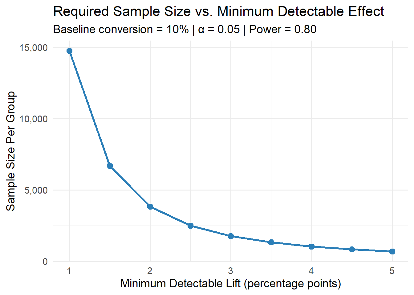
The curve is steep on the left: going from a 1pp lift to a 2pp lift cuts your required sample from roughly 15,000 to about 3,800 per group. But from 3pp to 5pp, the savings flatten out. This is the practical negotiation every team faces: if your site gets 1,000 visitors a day, detecting a 1pp lift means running the test for a month. Detecting a 3pp lift? About four days.
The takeaway for your planning: before you run your test, ask whether you can even afford to detect the effect you care about.
Now let’s see what an actual experiment looks like. We’ll generate fake data where we know the true effect — a 2 percentage point lift — and run a statistical test to see if we recover it. This is the advantage of simulation: we get to play god, then check whether our tools are good enough to find what we planted.
We use rbinom() to simulate each user’s conversion as a coin flip. Each user either converts (1) or doesn’t (0), with the probability set by the true conversion rate. The n argument is the number of users, size = 1 means each trial is a single yes/no outcome, and prob is the conversion rate:
set.seed(42)

n_per_group <- 3835
true_control_rate <- 0.10
true_treatment_rate <- 0.12

control   <- rbinom(n_per_group, size = 1, prob = true_control_rate)
treatment <- rbinom(n_per_group, size = 1, prob = true_treatment_rate)
set.seed(42) locks the random number generator so you get the same results we did. Without it, every run produces different simulated users — useful for exploration, but not for reproducible blog posts.
Now let’s look at what came out:
obs_control   <- mean(control)    # 0.1100
obs_treatment <- mean(treatment)  # 0.1244
obs_lift      <- obs_treatment - obs_control  # 0.0143
Notice something: we built in a 2pp lift, but observed only 1.43pp. The control rate came in at 11% instead of 10%. That’s not a bug — that’s sampling variability. With finite data, your observed rates will always wiggle around the true values. This is exactly why we need statistical tests: to figure out whether the wiggle is signal or noise.
We use prop.test() to run a two-proportion z-test. We pass in the number of successes and the number of trials for each group:
test_result <- prop.test(
  x = c(sum(treatment), sum(control)),
  n = c(n_per_group, n_per_group),
  correct = FALSE
)
We set correct = FALSE to skip the Yates continuity correction, which is conservative and generally unnecessary at sample sizes this large. The result:
p-value = 0.0509
95% CI: [-0.00005, 0.02874]
We failed to reject the null hypothesis. p = 0.0509, just barely above our α = 0.05 threshold. The confidence interval spans from essentially zero to 0.029 — it includes zero, so we can’t rule out no effect.
This is a perfect teaching moment. We built in a real 2pp effect, sized the test correctly, and still didn’t catch it. This is exactly what 80% power means: even when the effect is real and your sample size is right, you’ll fail to detect it 20% of the time. We just happened to land in that unlucky 20%.
A single test result is one draw from a distribution.
To really understand what 80% power feels like, let’s run the same experiment 1,000 times and count how often we correctly reject the null. This is a power simulation — the empirical version of what pwr.2p.test() calculated analytically.
This is where replicate() comes in. Think of it as “do this thing N times and give me back all the results.” It’s R’s clean way to repeat a random simulation. The first argument is how many times to repeat, and the second is the expression to evaluate each time. Here, each iteration simulates a full experiment — generate control data, generate treatment data, run the test, extract the p-value — and replicate() collects all 1,000 p-values into a single vector:
set.seed(123)

n_sims <- 1000
n_per_group <- 3835
true_control_rate <- 0.10
true_treatment_rate <- 0.12

p_values <- replicate(n_sims, {
  control   <- rbinom(n_per_group, 1, true_control_rate)
  treatment <- rbinom(n_per_group, 1, true_treatment_rate)
  test <- prop.test(
    x = c(sum(treatment), sum(control)),
    n = c(n_per_group, n_per_group),
    correct = FALSE
  )
  test$p.value
})
The curly braces { } inside replicate() let us run multiple lines as a single expression. Each pass through generates fresh random data (new simulated users with new coin flips), runs the hypothesis test, and returns just the p-value. After 1,000 passes, p_values is a numeric vector of length 1,000.
Now we check: out of those 1,000 experiments where the effect was real, how many times did we detect it?
empirical_power <- mean(p_values < 0.05)
# 0.813
81.3% empirical power, right in line with the theoretical 80%. The math works. But 187 out of 1,000 experiments missed the real effect — nearly 1 in 5.
The histogram of p-values makes this tangible:
df_pvals <- data.frame(p_value = p_values)

ggplot(df_pvals, aes(x = p_value)) +
  geom_histogram(bins = 40, fill = "#2c7fb8", color = "white", alpha = 0.8) +
  geom_vline(xintercept = 0.05, linetype = "dashed", color = "#e31a1c", linewidth = 1) +
  annotate("text", x = 0.08, y = max(table(cut(p_values, 40))) * 0.9,
           label = "α = 0.05", color = "#e31a1c", fontface = "bold", size = 5) +
  labs(
    title = "P-Value Distribution Across 1000 Simulated A/B Tests",
    subtitle = paste0("True effect exists (2pp lift) | Empirical power: ",
                      round(empirical_power * 100, 1), "%"),
    x = "P-Value", y = "Count"
  ) +
  theme_minimal(base_size = 14)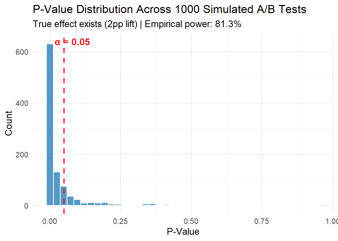
The p-values pile up hard against zero — that’s the test doing its job. But there’s a long right tail stretching past 0.05. Those are your missed detections: real effects that looked like noise.
Now flip the question. What happens when there’s no real effect and you test anyway? This is where false positives come from.
We run the same 1,000-experiment simulation, but this time both groups have the same 10% conversion rate:
set.seed(456)

n_sims <- 1000
null_rate <- 0.10

p_values_null <- replicate(n_sims, {
  control   <- rbinom(n_per_group, 1, null_rate)
  treatment <- rbinom(n_per_group, 1, null_rate)
  test <- prop.test(
    x = c(sum(treatment), sum(control)),
    n = c(n_per_group, n_per_group),
    correct = FALSE
  )
  test$p.value
})

mean(p_values_null < 0.05)
[1] 0.046# 0.046 — right at the expected 5%46 false discoveries out of 1,000. No real effect exists, but you’d have shipped a useless feature 46 times and celebrated each one.
Plotting both distributions side by side reveals the core mechanic:
df_both <- rbind(
  data.frame(p_value = p_values,      scenario = "Real Effect (2pp lift)"),
  data.frame(p_value = p_values_null, scenario = "No Effect (null true)")
)

ggplot(df_both, aes(x = p_value, fill = scenario)) +
  geom_histogram(bins = 40, color = "white", alpha = 0.7, position = "identity") +
  geom_vline(xintercept = 0.05, linetype = "dashed", color = "#e31a1c", linewidth = 1) +
  facet_wrap(~scenario, ncol = 1, scales = "free_y") +
  scale_fill_manual(values = c("#2c7fb8", "#fc8d59")) +
  labs(
    title = "P-Values: Real Effect vs. No Effect",
    subtitle = "Under the null, p-values are uniform — false positives happen at rate α",
    x = "P-Value", y = "Count"
  ) +
  theme_minimal(base_size = 14) +
  theme(legend.position = "none")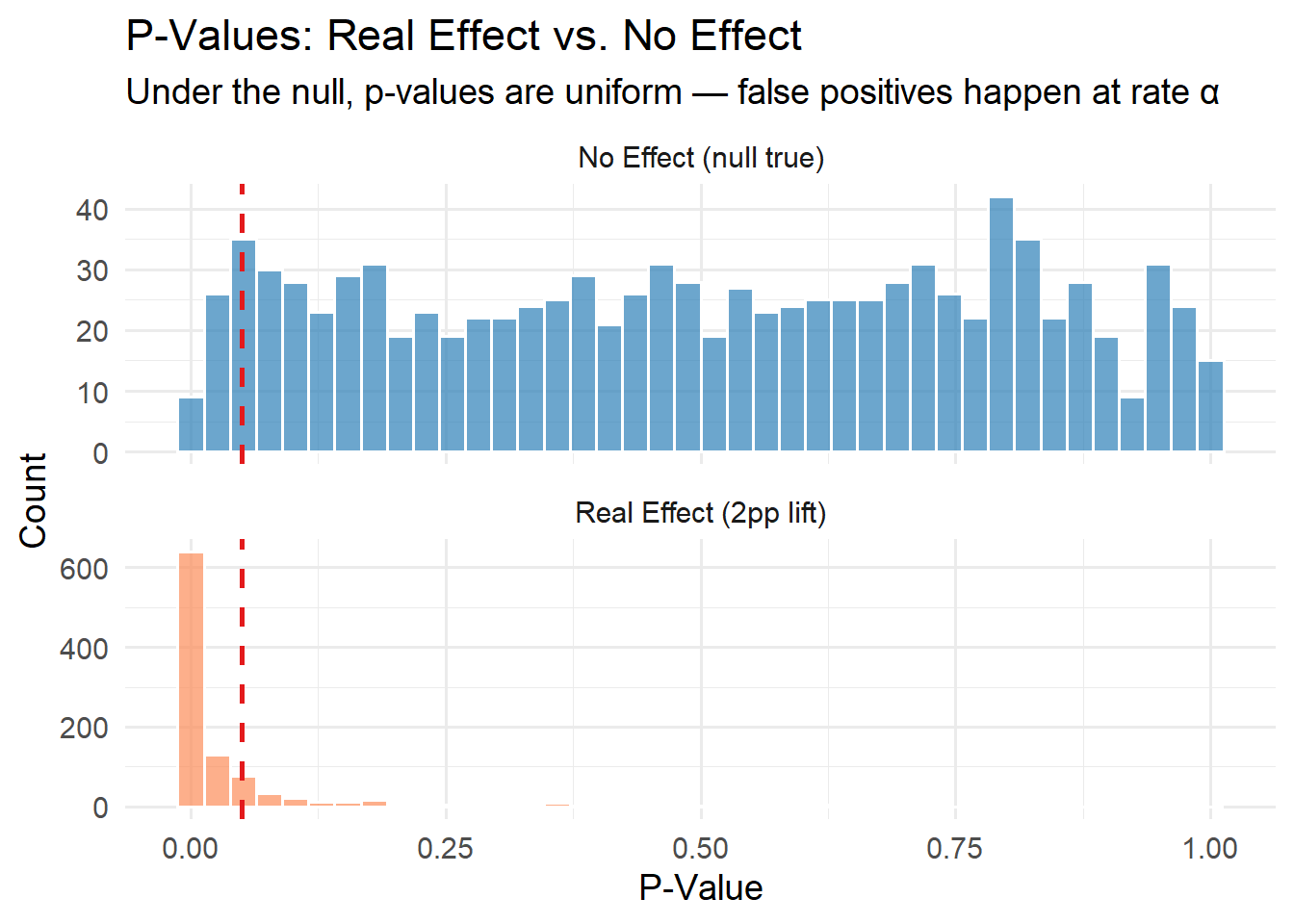
The “No Effect” panel shows p-values spread roughly uniformly from 0 to 1. That’s not a bug — it’s the definition of a well-calibrated test. When the null hypothesis is true, any p-value is equally likely. The ones that happen to fall below 0.05 are pure noise that you’d mistakenly act on.
The “Real Effect” panel shows the signal concentrating near zero. The contrast between these two panels is the whole foundation: when there’s a real effect, p-values cluster low. When there isn’t, they scatter everywhere, and α controls how much of that scatter you accidentally act on.
This is the pitfall that ruins more A/B tests than anything else, and it’s completely avoidable once you understand it.
Peeking is when someone checks results daily (or hourly, or whenever curiosity strikes) and stops the test the moment p drops below 0.05. It feels responsible — you’re monitoring your experiment! But it destroys your error guarantees.
Here’s why. Every time you look at accumulating data and ask “is it significant yet?”, you’re running another hypothesis test. Each test has a 5% chance of producing a false positive by design. Look 20 times, and you’ve given noise 20 chances to cross the line. The more you peek, the more likely one of those peeks will hit p < 0.05 by pure chance.
Let’s simulate it. We’ll run 1,000 experiments where there’s no real effect, but we check results every day for 20 days. If p < 0.05 on any day, we stop and declare a winner.
This simulation is more complex than our earlier ones because each experiment unfolds over time. Instead of generating all the data at once, we accumulate it day by day — each day adds 200 new users per group — and test at every step. The replicate() call wraps a for loop that walks through 20 days, and we use return() to exit early if we find significance:
set.seed(789)

n_sims <- 1000
daily_traffic_per_group <- 200
max_days <- 20
null_rate <- 0.10

peeking_decisions <- replicate(n_sims, {
  control_data   <- c()
  treatment_data <- c()

  for (day in 1:max_days) {
    control_data   <- c(control_data,   rbinom(daily_traffic_per_group, 1, null_rate))
    treatment_data <- c(treatment_data, rbinom(daily_traffic_per_group, 1, null_rate))

    test <- prop.test(
      x = c(sum(treatment_data), sum(control_data)),
      n = c(length(treatment_data), length(control_data)),
      correct = FALSE
    )

    if (test$p.value < 0.05) {
      return(c(rejected = 1, day_stopped = day))
    }
  }
  return(c(rejected = 0, day_stopped = max_days))
})
A few things to note about the code. We start with empty vectors (c()) and concatenate new data each day with c(control_data, rbinom(...)). This simulates accumulation — by day 10, control_data contains 2,000 observations (200 per day × 10 days). Each day’s prop.test() uses all accumulated data via length(treatment_data) rather than a fixed n, because the sample grows with each peek. The return() inside the for loop exits the entire replicate() expression early, mimicking a team that stops the experiment the moment they see significance.
The result of replicate() here is a 2 × 1000 matrix (two values per simulation — whether we rejected and which day we stopped). We transpose it into a data frame:
peeking_results <- as.data.frame(t(peeking_decisions))The results are damning:
False positive rate WITHOUT peeking: 5%
False positive rate WITH daily peeking: 24.6%
That's a 4.9x inflation!
24.6% false positive rate. Nearly 1 in 4 experiments would have been called a winner despite there being no real effect. And look at when the false positives happen:
Day stopped (among false positives):
 1  2  3  4  5  6  7  8  9 10 11 12 13 14 15 16 17 18 19 20
50 32 28 11 16 15 12  5  3 11  8  7  8  8  8  4  7  6  5  2
50 false positives on day 1 alone. With only 200 users per group, the estimates are wildly noisy, and random fluctuations cross p < 0.05 constantly. The early days are where peeking does the most damage.
One way to peek safely is to raise the bar for significance at each look. The Bonferroni correction divides your α budget equally across all planned peeks: if you’re going to look 20 times, require p < 0.05/20 = 0.0025 at each peek.
To show this, we need a slightly different simulation structure. Instead of stopping early, we record the p-value at every day for every experiment, then ask two questions after the fact: “Did the naive approach ever cross 0.05 by this day?” and “Did the corrected approach ever cross 0.0025 by this day?”
We use replicate() again, but this time the expression returns a vector of 20 p-values (one per day) instead of a single decision. The result is a 20 × 2000 matrix — each column is one simulated experiment, each row is a day:
set.seed(321)

n_sims <- 2000
alpha_bonferroni <- 0.05 / max_days  # 0.0025

sim_results <- replicate(n_sims, {
  control_data   <- c()
  treatment_data <- c()
  p_vals <- numeric(max_days)

  for (day in 1:max_days) {
    control_data   <- c(control_data,   rbinom(daily_traffic_per_group, 1, null_rate))
    treatment_data <- c(treatment_data, rbinom(daily_traffic_per_group, 1, null_rate))

    test <- prop.test(
      x = c(sum(treatment_data), sum(control_data)),
      n = c(length(treatment_data), length(control_data)),
      correct = FALSE
    )
    p_vals[day] <- test$p.value
  }
  p_vals
})
Now we compute the cumulative false positive rate at each day. The apply() call works column-by-column (each column is an experiment), slicing just the rows up to the current day with [1:day, , drop = FALSE] and checking if any p-value in that window crossed the threshold. The drop = FALSE is a defensive R habit — without it, subsetting a matrix to a single row drops it to a vector, which breaks apply():
fp_by_day_naive <- numeric(max_days)
fp_by_day_bonferroni <- numeric(max_days)

for (day in 1:max_days) {
  fp_by_day_naive[day] <- mean(apply(sim_results[1:day, , drop = FALSE], 2,
                                     function(x) any(x < 0.05)))
  fp_by_day_bonferroni[day] <- mean(apply(sim_results[1:day, , drop = FALSE], 2,
                                          function(x) any(x < alpha_bonferroni)))
}
Plotting both curves together:
df_fp <- data.frame(
  day = rep(1:max_days, 2),
  fp_rate = c(fp_by_day_naive, fp_by_day_bonferroni),
  method = rep(c("Naive (α = 0.05 each peek)",
                 paste0("Bonferroni (α = ", round(alpha_bonferroni, 4), " each peek)")),
               each = max_days)
)

ggplot(df_fp, aes(x = day, y = fp_rate, color = method)) +
  geom_line(linewidth = 1.2) +
  geom_point(size = 2.5) +
  geom_hline(yintercept = 0.05, linetype = "dashed", color = "gray40") +
  annotate("text", x = 15, y = 0.06, label = "Target: 5%", color = "gray40",
           fontface = "italic", size = 4.5) +
  scale_y_continuous(labels = scales::percent, limits = c(0, NA)) +
  scale_color_manual(values = c("#2c7fb8", "#e31a1c")) +
  labs(
    title = "Cumulative False Positive Rate: Naive Peeking vs. Bonferroni",
    subtitle = "No real effect | 200 users/group/day | Checked daily",
    x = "Day of Experiment",
    y = "Cumulative False Positive Rate",
    color = "Method"
  ) +
  theme_minimal(base_size = 14) +
  theme(legend.position = "bottom")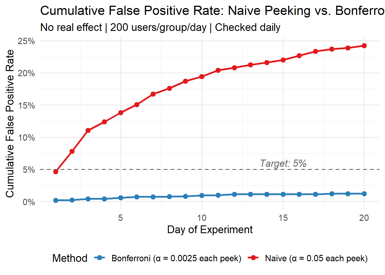
The red line (naive peeking) climbs to roughly 24% by day 20. The blue line (Bonferroni) stays well under 5% at about 1%. But that’s the trade-off: Bonferroni is too conservative. By requiring p < 0.0025, you’ll miss a lot of real effects. You’re buying error control at the cost of power.
In practice, the industry uses more sophisticated approaches — group sequential designs with O’Brien-Fleming or Pocock spending functions that distribute the alpha budget more intelligently across looks, or fully Bayesian monitoring. We’ll cover those in part 2.
Size your test first. Use pwr.2p.test() or power.prop.test() before you collect a single data point. If you can’t afford the sample size for the effect you care about, you can’t run the test.
A single test result is one draw from a distribution. Our correctly-sized experiment still missed the real effect because of sampling variability. An 80% power guarantee means 20% of the time, you’ll miss. That’s not a failure of the method — it’s the method telling you its limits.
Under the null, p-values are uniform. This is the most important thing to internalize. When nothing is happening, p-values scatter uniformly between 0 and 1, and 5% of them will be below 0.05 by pure chance. That’s not a coincidence — it’s literally the definition of α.
Don’t peek without correction. Daily peeking inflated our false positive rate from 5% to 25%. Either commit to a fixed sample size and don’t look until you hit it, or use a method designed for sequential monitoring.
Next up in Part 2: group sequential testing, Bayesian A/B testing with the BayesAB package, and when A/B testing is the wrong tool entirely.